Reinforcement Learning 101

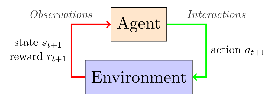
Reinforcement Learning (RL) is a field of research on the study of agents that can self-learn how to behave through feedback, reinforcement, from its environment, a sequential decision problem. RL is a subfield of Machine Learning, which in turn is a subfield of Artificial Intelligence or Computer Science.

RL differs from the more common machine learning task of Supervised Learning, wherein one is provided with a labeled dataset and has to infer a function that generalizes well on unseen examples. In RL, one starts without any such dataset and the agent has to obtain data through interaction in order to learn how to behave, and usually one intents to optimize the accumulated reward over the agent’s lifetime.

For example, let’s suppose we have a robot (our agent) that we send to Mars (the environment). We wish it to make a lot of distance and gather some rocks along the way. Although we could try to model the environment, it will require quite some resources and may be somewhat inaccurate. Controlling the robot from Earth is also not a good option, as our instructions will arrive minutes later. Thus, it might be a good idea to make our robot capable of learning by itself such that it can optimize its task.

Modelling the environment

Although the idea of RL is to avoid the necessity of modelling an environment, it is naturally very useful to model some environments in order to research how agents would behave and learn when they start from scratch.

In this blog post we will consider Markov decision processes. A Markov decision process (MDP) is an often-used discrete-time framework for modelling the dynamics of an environment (Howard, 1960; Puterman, 1994). A very explicit notation for an MDP is a sextuple $M = (\mathbb{S}, \mathbb{A}, P, R, I, \gamma)$, where

• $\mathbb{S}$ is the state space; the set of states that the MDP can be in. A state contains information regarding the environment. E.g., when flying a helicopter, a state pertains to the position and orientation of the helicopter. Let $s \in S$ denote a context-dependent state, and let $s_t$ denote the observed state at timestep $t$.
• $\mathbb{A}$ is the action space; the set of actions available to the agent. E.g., the pilot can choose to yaw, roll or pitch the helicopter. Let $a$ denote a context-dependent action, and let $a_t$ denote the action taken at $t$.
• $P : \mathbb{S} \times \mathbb{A} \times \mathbb{S} \to [0, 1]$; is a transition function that outputs a probability for a transition to a successor state after taking an action in a state. Let $S_t$ denote the random variable for the state at $t$, and $s'$ denote the immediate subsequent state. For each state $s$ and action $a$, the probability of transitioning to a successor state $s'$ respects constraints $Pr(s,a,s') \geq 0$ and $\sum_{s \in S} Pr(s,a,s') = 1$. The transition function basically determines what happens when an agent does something. E.g., after steering, the helicopter makes a turn.
• $R : \mathbb{S} \times \mathbb{A} \times \mathbb{S} \times \mathbb{R} \to [0, 1]$; is a reward function that outputs a probability for a numeric reward given a transition. Let $R_t$ denote the random variable for the reward at $t$, and let $r_t$ denote the observed reward at $t$. E.g., arriving at the destination incurs a high reward, and crashing incurs a negative reward.
• $I : \mathbb{S} \to [0, 1]$; is an initial state function that outputs the probability that a state is the MDPs initial state $s_0$. E.g., the helicopter can take off at several locations.
• $\gamma \in [0, 1]$; is a discount rate parameter that weighs off imminent rewards versus long-term rewards.

In the literature, one may find different notations. Commonly, no initial state function is mentioned, or the transition and reward functions are defined differently (or even notated as T). To the best of my knowledge, the above notation is the most explicit.

Actual implementations of MDPs employ datastructures of the programming language. For example, a numpy matrix with values between 0 and 1 describe the transition of a state-action pair (row) to a subsequent state (column).

At the beginning of interaction with an MDP, an agent observes an initial state $s_0$ and chooses an action $a_0$. From that point on, at each discrete timestep $t = 0, 1, 2, \dots$, it observes a successor state $s_{t+1}$ and a reward $r_{t+1}$, and chooses a new action accordingly.

Properties of MDPs

A stochastic MDP is an MDP where the transition function, reward function or initial state function is stochastic. Conversely, an MDP is deterministic when all three are deterministic. Notice that for a deterministic MDP, $S_t$ and $R_t$ can still be stochastic when actions are selected stochastically. Over time, the made observations and actions accumulate to a history. If the MDP or decision making is stochastic, then the resulting history is stochastic. We let $H_{0:t}$ denote the random variable over the history from timestep $0$ up to $t$ and define it as

$$H_{0:t} = \langle S_0, A_0, R_1, S_1, A_1, R_2, S_2, A_2, \dots, R_t, S_t \rangle$$

where $A_t$ is the random variable over the action taken at timestep $t$. The duration of the interaction is the horizon. If the interaction stops after a finite number of timesteps, we say the problem has a finite horizon and otherwise an infinite horizon. Some MDPs have terminal states, which divide interaction into episodes. Whenever a terminal state is reached, it ends the current episode and a new one starts by resetting the MDP to an initial state. E.g., a maze has an exit as terminal state. An MDP makes two important assumptions about the environment. First, it assumes that an agent can always perfectly observe the state of the environment. And second, it assumes that the Markov property holds (Howard, 1960; Puterman, 1994):

The future is conditionally independent of the past given the present.

Or mathematically, we note

$$Pr(R_{t+1}, S_{t+1} \vert S_t, A_t) = Pr(R_{t+1}, S_{t+1} \vert H_{0:t}, A_t)$$

We can exploit this assumption in both learning and decision making as we do not have to account for the past when we consider the present.

Types of MDPs and generalizations

A finite MDP has a finite state space and finite action space, and a continuous MDP has a continuous state space or action space. For an ergodic MDP, all states can be reached from all other states in a finite number of transitions. A stationary MDP is an MDP for which the parameters are fixed and independent of the timestep.

A partially observable Markov decision process (POMDP) does not assume that the state is perfectly observable and hence generalizes the MDP framework. This introduces an uncertainty over the state of the environment and complicates learning & decision making.

Multi-armed bandit problems can be considered as a special type of MDP: it always starts in the same state and each action leads to a terminal state. The name is inspired by one-armed bandits, which are machines found in casino’s where one pulls a lever in the hope of getting a winning combination (Sutton and Barto, 1998).

Policies and Objective Functions

In reinforcement learning, or rather decision making in general, one seeks to optimise an objective that is chosen prior to any interaction with the problem. For example: reaching a specific state or maximise some reward signal over the horizon.

We model the decision making of an agent as a policy function, or policy, and denote it by $\pi$. In its most general form, a policy maps histories and actions to probabilities:

$$\pi : \mathbb{H} \times \mathbb{A} \to [0, 1]$$

where $\mathbb(H)$ is the space of all possible histories. For an MDP, it suffices that a policy is a mapping from states and actions to probabilities (thankfully!). A Markovian policy is defined as:

$$\pi : \mathbb{S} \times \mathbb{A} \to [0, 1] .$$

At each timestep, an agent will choose a single action available in the current state according to its probability,

$A_t \sim \pi(H_{0:t}, \cdot)$ or $A_t \sim \pi(S_t, \cdot)$

which can be interpreted as the agent’s preference for that action.

A policy is stochastic when in some state more than one action has a non-zero probability of being selected. Conversely, a deterministic policy has in each state a single action with probability one. In other words you could then also define the policy as a function that maps states to actions.

For a learning agent, its preference over actions can change over time and is therefore time-dependent and typically not Markovian as it is the result of the history. We use $\Pi$ to denote the set of all policies.

Objective Functions

The performance of a policy $\pi$ on a MDP $M$ is measured using an objective function. In the literature of reinforcement learning, one commonly wants to maximize the expected sum of discounted rewards, or expected return [C. Szepesvari, 2010]. The expected return of a $\pi$ on an $M$ for an infinite horizon is defined by

$$J(\pi, M) = \mathbb{E}_{\pi, M} \{ \sum_{t=0}^{\infty} \gamma^t R_t \}$$

where $\sum_{t=0}^{\infty} \gamma^t R_t$ functions as a single random variable called the return, which depends on the stochasticity of rewards, transitions, initial state and the policy. Here I use $\mathbb{E}_{\pi, M} \{ X \}$ to denote an expectation of a random variable $X$ when following $\pi$ on $M$.

The discount rate parameter, $\gamma \in [0, 1]$, weighs off immediate rewards versus long-term rewards [Sutton and Barto, 1998]. I.e., a reward received $n$ steps in the future only contributes $\gamma^n$ of that reward. As $\gamma$ goes to one, future rewards contribute more.

Conceptually, $J(\pi, M)$ represents the value of a policy. An objective function thus enables one to compare and prefer policies based on their values. A policy that optimises the objective function is called an optimal policy, and is commonly denoted by $\pi^*$. For any MDP, a deterministic Markovian $\pi^*$ always exists [Puterman, 1994]. For the expected return over an infinite horizon, it is obvious that $\pi^*$ has the maximal possible value:

$$\pi^* = \arg\max_{\pi \in \Pi} J(\pi, M) .$$

In reinforcement learning, we often want to address the problem of control: finding an optimal policy which optimises the chosen objective function. The problem of prediction, which is also known as policy evaluation in the literature, is about estimating the value of a policy $J(\pi, M)$. Naturally, one can use the latter to solve the former: we can compare and choose the policy with the highest value.

Comparing Reinforcement Learning Algorithms

Although I have not discussed any RL algorithm yet, I think it is very important to understand the concepts in this section. This is something that might also be of interest to OpenAI/Gym. In order to correctly compare RL algorithms, it is important to understand the (in my opinion often-forgotten) distinction between online versus offline reinforcement learning [H. van Hasselt. 2011].

Consider the following, when developing learning agents, one can distinguish between a learning phase and a deployment phase. During the learning phase, the agent tries out actions, learns and infers a good policy for the environment that it can subsequentially follow during the deployment phase, where the agent’s performance matters. Note that the learning phase may very well happen within the same environment as the deployment phase. In RL one also distinguishes between an estimation policy, the policy one learns about, and the behaviour policy, that the agent uses for interaction with the environment. Algorithms for RL can thus be on-policy when the estimation policy is the same as the behaviour policy, or off-policy when they are different.

In offline reinforcement learning, one learns a policy during the learning phase for some predetermined time and then measures the learned policy’s performance during deployment. This differs from online reinforcement learning where one measures the performance of the behaviour policy. Or in other words, the learning and deployment phase occur simulatenously. Evidently, an agent that starts from scratch will perform poorly in the initial stages and it becomes very important to balance between exploring an unknown but potentially good action and exploiting known good actions. This is known under various names: exploration versus exploitation dilemma, balancing exploration with exploitation, and the exploration-exploitation trade-off.

In the literature, the most common approach to measuring and comparing in experiments (as well as in OpenAI/Gym) is to measure the performance of the behaviour policy over a finite timesteps (or episodes) and average over a number of timesteps.

Afterword

I hope you learned a bit about reinforcement learning from this blog post.

In future blogs, I intent to discuss

• Value functions, and the learning thereof.
• Exploration-vs-Exploitation in MDPs
• Difficulties & Troubleshooting RL implementations

and, of course, code for you to try yourself!

Feel free to suggest topics!

References

[Howard, 1960] R.A. Howard. Dynamic programming and Markov processes. MIT Press, 1960.

[Puterman, 1994] M.L. Puterman. Markov Decision Processes: Discrete Stochastic Dynamic Programming. John Wiley & Sons, Inc. new York, NY, USA, 1994.

[Sutton and Barto, 1998] R.S. Sutton and A.G. Barto. Reinforcement Learning: An Introduction (Adaptive Computation and Machine Learning). The MIT Press, 1998.

[C. Szepesvari, 2010] Algorithms for Reinforcement Learning. Synthesis Lectures on Artificial Intelligence and Machine Learning. Morgan & Claypool, 2010.

[H. van Hasselt. 2011] Insights in Reinforcement Learning. PhD thesis, Utrecht University, 2011.