Learning Value Functions

Value Functions

In this blog post we gonna talk about one of my favorite parts of reinforcement learning: Value Functions. The first parts will look difficult and kinda mathemetical, but they will give you a good basis to understand how the different learning algorithms are derived.

A value function maps each state to a value that corresponds with the output of the objective function. We use $V_{M}^{\pi}$ to denote the value function when following $\pi$ on $M$ , and let $V_{M}^{\pi}(s)$ denote the state-value of a state $s$ . In the literature $M$ is often omitted as it is clear from context. A state-value for the expected return of a policy on $M$ is defined by

$V_{M}^{\pi}(s) = \mathbb{E}_{\pi, M} \{ \sum_{k=0}^{\infty} \gamma^k R_{t+k+1} \vert S_t = s \}$

where $\mathbb{E}_{\pi, M} \{ X \vert Y \}$ is the conditional expectation of $X$ given $Y$ when following $\pi$ on $M$ . Thus, a state-value indicates how good it is to be in its respective state in terms of the expected return. If we want to perform well, we prefer states with high state-values.

The value function of the optimal policy, $\pi^*$ is called the optimal value function and is denoted by $V_{M}^{\pi^*}$ and in the literature usually just $V^*$ . Evidently, it holds that for each state, $V^*(s)$ is equal or higher than for other policies:

$\forall_{\pi \in \Pi, s \in \mathbb{S}} : V^*(s) \geq V^{\pi}(s)$

Q-functions

An action-value function or more commonly known as Q-function is a simple extension of the above that also accounts for actions. It is used to map combinations of states and actions to values. A single combination is often referred to as a state-action pair, and its value as a (policy) action-value.

We use $Q_{M}^{\pi}$ to denote the Q-function when following $\pi$ on $M$ , and let $Q_{M}^{\pi}(s,a)$ denote the action-value of a state-action pair $(s,a)$ . In the literature, it is common to leave out both $\pi$ and $M$ . The action-value is then:

$Q_{M}^{\pi}(s,a) = \mathbb{E}_{\pi, M} \{ \sum_{k=0}^{\infty} \gamma^k R_{t+k+1} \vert S_t = s, A_t = a \}$

which corresponds to the idea that when you are in state $s$ and take $a$ and follow $\pi$ afterwards then the expectation is as above.

The Q-function of $\pi^*$ is called the optimal Q-function. It is usually noted as $Q^*$ . Notice that state-values and action-values are related to each other as follows:

$V^{\pi}(s) = \sum_{a\in\mathbb{A}}\pi(s,a)Q^{\pi}(s, a)$ and $V^*(s) = max_{a\in\mathbb{A}}Q^*(s, a)$

Deriving policies from Q-functions

It is very straightforward to derive policies from Q-functions as they describe how good each action is. In the literature, the most common derivation is the greedy policy of a Q-function: in each state, choose the greedy action, which is the action with the highest action-value. Notice that we can derive $\pi^*$ by using a greedy policy with respect to $Q^*$ *. Also notice that $Q^*$ is sufficient but not necessary for $\pi^*$ : any of the action-value actions can be changed as long as the same best actions keep the highest action-values.

Q-functions are frequently used to guide exploration and exploitation. The most common approach is to use epsilon-greedy: at each timestep, choose a greedy action with probability $1-\epsilon$ or choose a random action with probability $\epsilon$ [Sutton and Barto, 1998]. Interestingly, in the literature never considers the case that a random action might still choose the same greedy action and hence the chance of choosing the greedy action is usually higher than $1-\epsilon$ . When using epsilon-greedy, one commonly starts with a high $\epsilon$ and decrease it over a time. Evidently, when $\epsilon = 0$ , it is equal to the greedy policy.

Another approach I like to mention is Boltzmann exploration, where one introduces a temperature parameter $\beta$ to map action-values to action probabilities as follows:

$Pr(a) = \frac{exp(Q(s,a) / \beta)}{\sum_{b \in \mathbb{A}} exp(Q(s,a) / \beta)}$

The parameter is used to control how the difference in action-values corresponds to a difference in action-probabilities. As $\beta$ goes to zero, Boltzmann chooses greedily, and as $\beta$ goes to infinity, all actions have an equal chance. In different research fields this formula is also known as softmax.

Bellman Equations

For MDPs, action-values (and state-values) share an interesting recursive relation between them, clarified by the so-called Bellman equation [Bellman, 1957]. The Bellman equation for an action-value is derived as follows:

$\begin{align} Q_{M}^{\pi}(s,a) &= \mathbb{E}_{\pi, M} \{ \sum_{k=0}^{\infty} \gamma^k R_{t+k+1} \vert S_t = s, A_t = a \} \\ &= \mathbb{E}_{\pi, M} \{ R_{t+1} + \gamma R_{t+2} + \gamma^2 R_{t+3} + \dots \vert S_t = s, A_t = a \} \\ &= \mathbb{E}_{\pi, M} \{ R_{t+1} + \gamma V^{\pi}(S_{t+1}) \vert S_t = s, A_t = a \} \\ &= \mathbb{E}_{\pi, M} \{ R_{t+1} + \gamma \sum_{a'\in\mathbb{A}}\pi(S_{t+1},a')Q^{\pi}(S_{t+1}, a') \vert S_t = s, A_t = a \} \end{align}$

The Bellman equation version for $\pi^*$ is called the Bellman optimality equation, and is formulated as

$\begin{align} Q_{M}^{*}(s,a) &= \mathbb{E}_{\pi^*, M} \{ R_{t+1} + \gamma V^{*}(S_{t+1}) \vert S_t = s, A_t = a \} \\ &= \mathbb{E}_{\pi^*, M} \{ R_{t+1} + \gamma \sum_{a'\in\mathbb{A}}Q^{*}(S_{t+1}, a') \vert S_t = s, A_t = a \} \end{align}$

Clearly, an action-value can be alternatively defined as the expectation over immediate rewards and the action-values of successor state-action pairs. Reinforcement learning algorithms commonly exploit these recursive relations for learning state-values and action-values.

Temporal-Difference Learning

Temporal-difference (TD) learning algorithms bootstrap value estimates by using samples that are based on other value estimates as inspired by the Bellman equations [Sutton and Barto, 1998]. We will only consider estimates for action-values by using Q-functions.

Let $Q_t$ denote a Q-function estimate at timestep $t$ , where $Q_0$ is arbitrarily initialized. In general, a TD algorithm updates the action-value estimate of the state-action pair that was visited at timestep $t$ , denoted by $Q_t(S_t, A_t)$ , as follows

$Q_{t+1}(S_t, A_t) = Q_t(S_t, A_t) + \alpha_t (X_t - Q_t(S_t, A_t))$

where $Q_{t+1}(S_t, A_t)$ is the updated action-value estimate, and $X_t$ is a value sample observed at $t$ and is based on different mechanisms in the literature. The learning rate $\alpha_t \in [0, 1]$ weighs off new samples with previous samples.

The above TD-learning algorithm is commonly implemented in an online manner: whenever the agent takes an action and observes reward $r_{t+1}$ and transition to next state $s_{t+1}$ , a value sample $X_t$ is constructed and the relevant estimate (of the previous state-action pair) is updated. Once updated, the sample is discarded.

Below a short list of different value samples used by different RL algorithms:

Algorithm	Value Sample
Q-learning	$X_t = R_{t+1} + \gamma \max_{a' \in \mathbb{A}} Q_t(S_{t+1}, a')$
SARSA	$X_t = R_{t+1} + \gamma Q_t(S_{t+1}, a')$
Expected SARSA	$X_t = R_{t+1} + \gamma \sum_{a' \in \mathbb{A}} \pi_t(S_{t+1},a') Q_t(S_{t+1}, a')$
Double Q-learning	$X_t = R_{t+1} + \gamma \max_{a' \in \mathbb{A}} Q_t^b(S_{t+1}, a')$

where $Q_t^b$ is the second Q-function, see Double Q-learning. Notice that Q-learning and Double Q-learning are off-policy: they learn about a different (implicit) policy than the behaviour policy used for interaction. SARSA and Expected SARSA are on-policy: they learn about the same policy as the agent follows.

Bias and Variance

Despite that sample rewards and transitions are unbiased, the value samples used by TD algorithms are usually biased as they are drawn from a bootstrap distribution. Namely, estimates are used instead of the true action-values:

$Q_t(S_{t+1}, \cdot)$ instead of $Q^*(S_{t+1}, \cdot)$ or $Q^\pi(S_{t+1}, \cdot)$

However, bootstrapping has several advantages. First, we do not need to wait until we have a sample return, consisting of a(n infinite) number of sample rewards, before we can update estimates. This can tremendously improve the speed with which we learn. Second, we need to know the true action-values (or the optimal policy) to obtain unbiaased samples, which are simply not known. Third, the bootstrap distribution’s variance is smaller than the variance of the distribution over whole returns.

A second bias occurs when we change the implicit estimation policy towards an action that is perceived as better than it actually is. I.e., for Q-learning, we estimate the optimal action-value based on the maximum action-value estimate [van Hasselt, 2011] :

$max_{a \in \mathbb{A}} Q_t(S_{t+1}, a)$ instead of $Q_t(S_{t+1}, a*)$

where $a*$ denotes the optimal action in the successor state. This overestimation bias becomes apparent when we severely overestimate action-values of suboptimal actions, due to an extremely high value sample or improper initialization. As a result, other estimates can also become overestimated as value samples will be inflated due to bootstrapping, and may remain inaccurate as well as mislead action-selection for an extended period of time. Double Q-learning addresses this overestimation bias, but may suffer from an underestimation bias instead [van Hasselt, 2011]

Learning Rates

The learning rate $\alpha_t$ is used to weigh off new value samples with previous value samples. There are many schemes available for the learning rate. For example, if the MDP is deterministic we can set the learning rate at one at all times. Usually, the MDP is stochastic and a lower value than one should be used. For instance, one can use a hyperharmonic learning rate scheme:

$\alpha_t(s,a) = \frac{1}{n_t(s,a)^w}$

where $n_t(s,a)$ is the number of times $(s,a)$ has been visited by timestep $t$ , and $w \in (0.5, 1]$ is a tunable parameter of the scheme. [Even-Dar and Mansour, 2003]showed that $0.5 < w < 1$ (hyperharmonic) works better than $w = 1$ (harmonic). This is because the value samples are based on other estimates that may change over time, and hence the distribution of the value samples are non-stationary as well as not independent and identically distributed (not i.i.d.).

Convergence

Q-learning and the other above-mentioned choices are proven to converge to the optimal Q-function in the limit with probability one [van Hasselt, 2011]. Provided that a few conditions are satisfied:

The behaviour policy guarantees that every state-action pair is infinitely often tried in the limit.
The learning-rate satisfies the Robbin-Monro’s conditions for stochastic approximation: $\sum_{t=0}^{\infty} \alpha_t = \infty$ and $\sum_{t=0}^{\infty} (\alpha_t)^2 < \infty$
for Sarsa and Expected Sarsa, the estimation policy (and hence behaviour policy) is greedy in the limit.

Put simply, the easiest way to guarantee convergence: use a simple learning rate as mentioned above, initialize however you want, and use epsilon-greedy where $\epsilon$ is above $0$ (already satisfied by doing $\epsilon = 1/t$ ).

Python Implementations

Q-learning

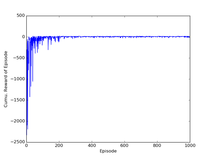
For a discrete problem, the following python implementation of Q-learning works well enough:

import gym
env = gym.make("Taxi-v1")


# Q-function
# initial_Q = 0.
from collections import defaultdict
Q = defaultdict(lambda : 0.) # Q-function
n = defaultdict(lambda : 1.) # number of visits


# Extra
actionspace = range(env.action_space.n)
greedy_action = lambda s : max(actionspace, key=lambda a : Q[(s,a)])
max_q = lambda sp : max([Q[(sp,a)] for a in actionspace])
import random
epsilon = 0.1
gamma = 0.9


# Simulation
episodescores = []
for _ in range(500):
    nextstate = env.reset()
    currentscore = 0.
    for _ in range(1000):
        state = nextstate

        # Epsilon-Greedy
        if epsilon > random.random() :
            action = env.action_space.sample()
        else :
            action = greedy_action(state)

        nextstate, reward, done, info = env.step(action)
        currentscore += reward

        # Q-learning
        if done :
            Q[(state,action)] = Q[(state,action)] + 1./n[(state,action)] * ( reward - Q[(state,action)] )
            break
        else :
            Q[(state,action)] = Q[(state,action)] + 1./n[(state,action)] * ( reward + gamma * max_q(nextstate) - Q[(state,action)] )

    episodescores.append(currentscore)


import matplotlib.pyplot as plt
plt.plot(episodescores)
plt.xlabel('Episode')
plt.ylabel('Cumu. Reward of Episode')
plt.show()

This code resulted in the following performance:

Q-learning

SARSA

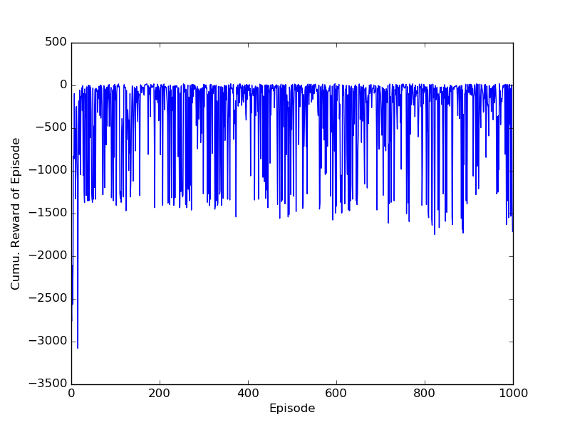
Also, a simple implementation of SARSA:

import gym
env = gym.make("Taxi-v1")


# Q-function
# initial_Q = 0.
from collections import defaultdict
Q = defaultdict(lambda : 0.) # Q-function
n = defaultdict(lambda : 1.) # number of visits


# Extra
actionspace = range(env.action_space.n)
greedy_action = lambda s : max(actionspace, key=lambda a : Q[(s,a)])
import random
epsilon = 0.1
gamma = 0.9


# Simulation
episodescores = []
for _ in range(500):
    state = env.reset()
    currentscore = 0.
    for t in range(1000):
        # Epsilon-Greedy
        if epsilon > random.random() :
            action = env.action_space.sample()
        else :
            action = greedy_action(state)

        # SARSA
        if t > 0 : # Because previous state and action do not yet exist at t=0
            Q[(prevstate,prevaction)] = Q[(prevstate,prevaction)] + 1./n[(prevstate,prevaction)] * ( reward + gamma * Q[(state, action)] - Q[(prevstate,prevaction)] )

        nextstate, reward, done, info = env.step(action)
        currentscore += reward

        if done :
            Q[(prevstate,prevaction)] = Q[(prevstate,prevaction)] + 1./n[(state,action)] * ( reward - Q[(prevstate,prevaction)] )
            break

        prevstate, state, prevaction = state, nextstate, action

    episodescores.append(currentscore)


import matplotlib.pyplot as plt
import numpy as np
plt.plot(episodescores)
plt.xlabel('Episode')
plt.ylabel('Cumu. Reward of Episode')
plt.show()

And the resulting image. Notice that the performance does not seem to converge to the optimal, this is because SARSA is on-policy and the behaviour-policy remains epsilon-greedy with $\epsilon = 0.1$ and thus will do a random (bad) action roughly 10% of the time.

SARSA

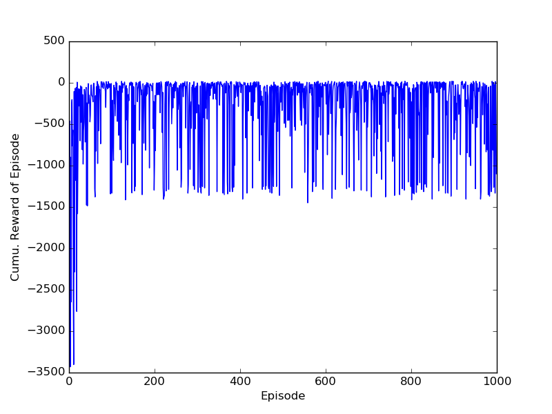
Expected SARSA

import gym
env = gym.make("Taxi-v1")


# Q-function
# initial_Q = 0.
from collections import defaultdict
Q = defaultdict(lambda : 0.) # Q-function
n = defaultdict(lambda : 1.) # number of visits


# Extra
actionspace = range(env.action_space.n)
greedy_action = lambda s : max(actionspace, key=lambda a : Q[(s,a)])
import random
epsilon = 0.1
gamma = 0.9


# Simulation
episodescores = []
for _ in range(1000):
    state = env.reset()
    currentscore = 0.
    for t in range(1000):
        # Epsilon-Greedy
        if epsilon > random.random() :
            action = env.action_space.sample()
        else :
            action = greedy_action(state)

        # Expected SARSA
        if t > 0 : # Because previous state and action do not yet exist at t=0
            Vpi = sum([ Q[(state, a)] * ((action==a)*(1.-epsilon) + epsilon*(1./len(actionspace))) for a in actionspace ])
            Q[(prevstate,prevaction)] = Q[(prevstate,prevaction)] + 1./n[(prevstate,prevaction)] * ( reward + gamma * Vpi - Q[(prevstate,prevaction)] )

        nextstate, reward, done, info = env.step(action)
        currentscore += reward

        if done :
            Q[(prevstate,prevaction)] = Q[(prevstate,prevaction)] + 1./n[(state,action)] * ( reward - Q[(prevstate,prevaction)] )
            break

        prevstate, state, prevaction = state, nextstate, action

    episodescores.append(currentscore)


import matplotlib.pyplot as plt
import numpy as np
plt.plot(episodescores)
plt.xlabel('Episode')
plt.ylabel('Cumu. Reward of Episode')
plt.show()

And its performance: Expected SARSA

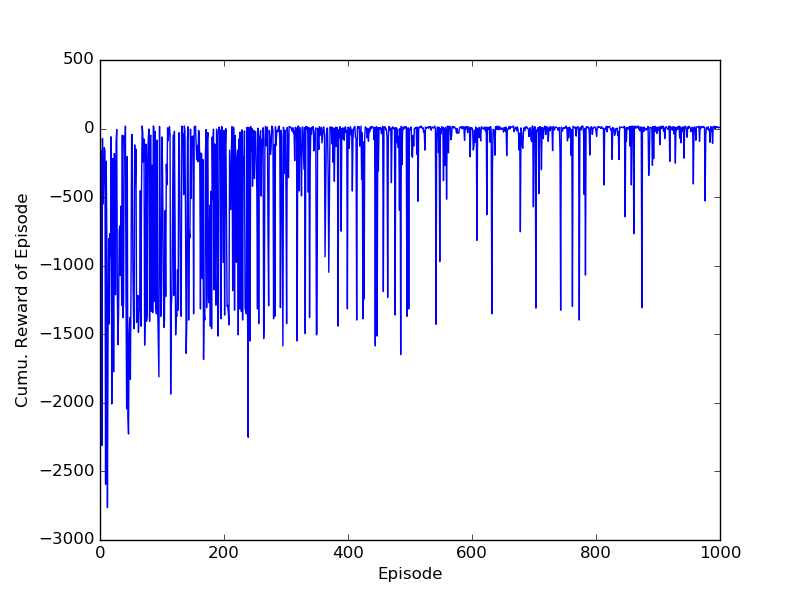
Double Q-learning

Code:

import gym
env = gym.make("Taxi-v1")


# Q-function
# initial_Q = 0.
from collections import defaultdict
Q = defaultdict(lambda : 0.) # Q-function
n = defaultdict(lambda : 1.) # number of visits


# Extra
actionspace = range(env.action_space.n)
greedy_action_i = lambda i, s : max(actionspace, key=lambda a : Q[(i,s,a)])
max_q = lambda i, sp : max([Q[(i,sp,a)] for a in actionspace])
greedy_action = lambda s : max(actionspace, key=lambda a : (Q[(0,s,a)]+Q[(1,s,a)])/2.)
import random
epsilon = 0.1
gamma = 0.9


# Simulation
episodescores = []
for _ in range(1000):
    nextstate = env.reset()
    currentscore = 0.
    for _ in range(1000):
        state = nextstate

        # Epsilon-Greedy
        if epsilon > random.random() :
            action = env.action_space.sample()
        else :
            action = greedy_action(state)

        nextstate, reward, done, info = env.step(action)
        currentscore += reward

        # Double Q-learning
        i = random.choice([0,1])
        o = (i + 1) % 2
        if done :
            Q[(i,state,action)] = Q[(i,state,action)] + 1./n[(i,state,action)] * ( reward - Q[(i,state,action)] )
            break
        else :
            greedy_i = greedy_action_i(i,nextstate)
            Q[(i,state,action)] = Q[(i,state,action)] + 1./n[(i,state,action)] * ( reward + gamma * Q[(o,nextstate,greedy_i)] - Q[(i,state,action)] )

    episodescores.append(currentscore)


import matplotlib.pyplot as plt
plt.plot(episodescores)
plt.xlabel('Episode')
plt.ylabel('Cumu. Reward of Episode')
plt.show()

And the performance: Double Q-learning

Afterword

We have discussed value-functions and a few simple temporal-difference learning algorithms, and demonstrated their implementation and some performance. Although SARSA and Expected SARSA look like they perform poorly, they certainly are not always worse than Q-learning. It just so happens that the Taxi environment works quite well with the chosen epsilon-greedy action-selection. In other environments, SARSA and Expected SARSA may perform much better than Q-learning, namely environments were a single mistake inflicts a devastating reward feedback. For example when walking alongside a cliff, the on-policy approach will then take into account the chance that one sometimes randomly wanders off the cliff if it walks too close along the cliff and hence induces a safer policy [Sutton and Barto, 1998].

Next topic is on Advanced Value Functions.

References

[Bellman, 1957] R. Bellman. Dynamic Programming. Princeton University Press, 1957.

[Even-Dar and Mansour, 2003] E. Even-Dar and Y. Mansour. Learning rates for Q-learning. The Journal of Machine Learning Research, 5:1–25, 2003.

[Sutton and Barto, 1998] R.S. Sutton and A.G. Barto. Reinforcement Learning: An Introduction (Adaptive Computation and Machine Learning). The MIT Press, 1998.

[H. van Hasselt. 2011] Insights in Reinforcement Learning. PhD thesis, Utrecht University, 2011.

Written on August 21, 2016